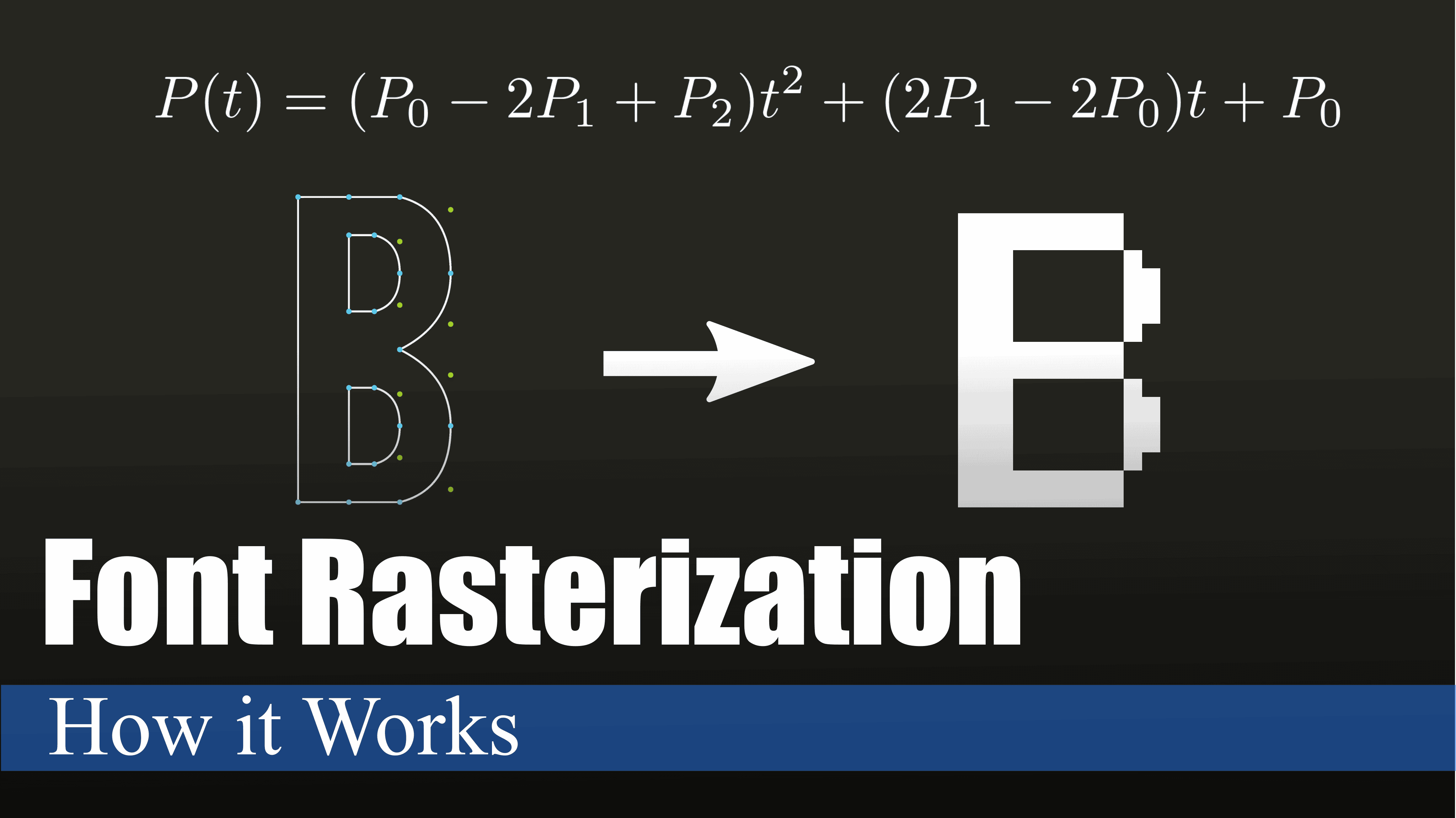
The Math Behind Font Rasterization

If you have ever written a document, read a book, made a PowerPoint presentation, built a website, or worked with text in general, then you have used font rasterization. Font rasterization is the process of converting a vector description to a raster or bitmap description. In other words, font rasterization is converting mathematical formulas to pixels on the screen you are using. We use this process everyday when we use our phones, but have you ever wondered how it really works?

(If you prefer videos to articles, you can watch this article in video format here)

A Brief History of Fonts

Computers display graphics to us by using pixels on a screen. In the 80’s and 90’s we had very limited resolutions because computing power was not sufficient enough to support many pixels on the screen. Now, we have resolutions that contain upwards of 33 million pixels on a screen. Compared to a Nintendo Gameboy, which only has 23 thousand pixels on the screen, that is insane. Now, why are we discussing pixels and screen resolutions? Because in order to understand the evolution of font rasterization you must understand where we came from, and where we are now.

If I asked you how to represent text using a limited number of pixels, how would you do it? Well, the easiest way I could think of would be to simply plot the pixels in the shape of letters. This is simple and straightforward, and it is very easy to communicate to a computer that deals with pixels. So, plotting the letters ‘A’, ‘B’, and ‘C’ would look something like this:

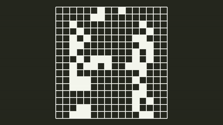
We can very easily calculate how much computer memory this would take up per character set. If we assume each pixel is represented by 8-bits (allowing a grayscale image to add some variety), and each letter is only 32x32 pixels, then storing the English alphabet would only take up \((8 *32* 32 *26* 2) = 425,984\) bits (we do \(26 * 2\) for the 26 letters in the English alphabet in lowercase and uppercase). We know that one byte is 8 bits, so this would take up 53,284 bytes or around 53 kilobytes. This is great, we can store an alphabet in a way that’s easy to communicate to the computer, and it also takes up very little space on the computer.

But there’s one problem, what if we want a different font size? Unfortunately, our whole technique breaks down here. The process I just described is how the bitmap file format works, which was created around 1986. This file format is a more complex version of the process that I described above. It stores fonts in a file by essentially storing the pixel data itself. Around 1991 Apple decided to add support for a new font file format that would solve our problem, the TrueType file format. So, we must revisit our original question.

If I asked you how to represent text using an unknown number of pixels, how would you do it? Before we assumed you knew how many pixels you could use, and it was limited. But now let’s assume that the user could use a 12 pixel font size, or a 512 pixel font size. How do you represent the letter ‘A’ for both of those? Well you could create a bitmap file for both pixel sizes and switch the file for different sizes, but this is very inefficient and costly. A 512 pixel font size for the English alphabet would take 109,051,904 bits, or around 13.3 megabytes. We are now wasting a lot of memory for the different font sizes, and we are multiplying the amount of work for ourselves by having to recreate the font for every font size. Instead, let’s use math to solve this problem.

Using Math to Draw Letters

We know that you can represent curves in math using an equation. There are different kinds of curves that you can create. For example, here are some simple curves.

We can also translate these curves by adding offsets to our equations. We can offset a quadratic curve vertically by adding a number outside the equation, and horizontally by adding a number inside the equation. We can do all sorts of transformations to our curve by modifying it slightly to get different results.

Now we know two things:

1. We can represent any curve using an equation.
2. A letter is just a combination of several different types of curves.

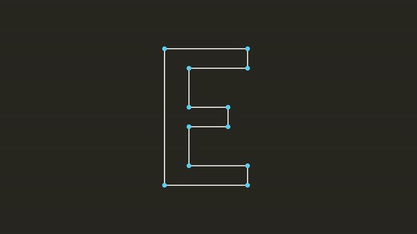
Now that we know this, we can set out to represent a font as a series of mathematical curves that describe each letter. But how do we do this? We could define a set of points that we want our curve to pass through. Then we could connect each of these points with a straight line, but for letters like ‘C’ this won’t work very well because of the curvature.

We could define a polynomial to pass through each of these points, and there are entire procedures to do this. One of these procedures is known as Lagrange Interpolation which will create a polynomial that will pass through all of your points. But this doesn’t give sharp edges that are expected in a letter like ‘A’. So we have two techniques that work for different types of letters, why don’t we combine them?

Lagrange Interpolation

That’s exactly the process that the TrueType file format takes. It combines straight lines and simple 2nd order Bézier curves to describe a set of letters. A Bézier curve is special because it can represent a curve using a set of control points \(P_0\) through \(P_n\). Where \(P_0\) and \(P_n\) are the endpoints, and all the in between points are control points. These control points describe how the curve should “bend”, and if we keep it simple with 2nd order Bézier curves, then we only ever have 3 points to describe a curve that bends in one direction.

Bézier Curve

Now we have a solution. We can represent the outline of a letter using a series of points and a description that tells us whether the next two points are a line, or the next three points are a Bézier curve.

We have another problem though. Sure we can draw the outline of the shape, but this does not help us draw “solid” letters. Remember that computers are made of discrete pixels and all we have is a way to describe a series of curves that describes an outline of a letter. How do we fill the letter in? Well, the simplest way we could do this is by drawing the outline first. This will give us a closed set of pixels which outline the letter. Once we have the outline drawn, we can simply pick a pixel “inside” the letter and “fill” the shape from there.

Flood Filling a Letter

This will work fairly well, however when we get to a complex letter like “B” we run into another problem. What is considered the “inside” of the letter? We intuitively know that it’s these pixels:

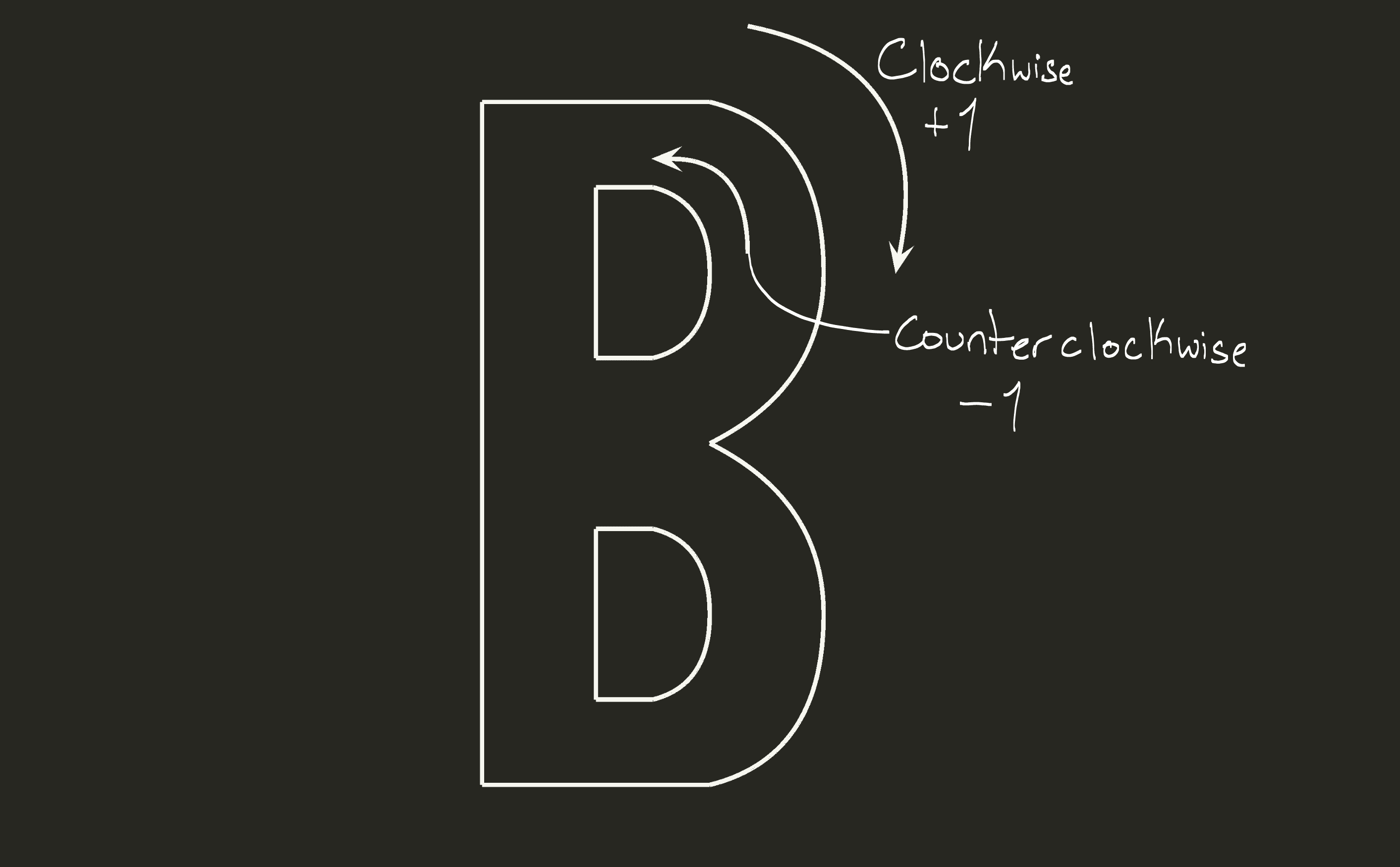
But how does the computer know it’s these pixels and not the pixel inside the holes as well? Well, some clever mathematicians have already solved this for us. Let’s look at this problem from another angle. Instead of drawing the outline, why don’t we “test” each pixel to determine whether it is inside the outline or outside the outline. If we think about it this way we can come up with a solution that should work. Notice that with the letter “B” we can look at a pixel over here, and if we draw a line to the right how many times do we hit a line?

Well we run into 4 lines. What about when we start inside here?

We run into three lines. There’s a pattern here. Every time a pixel is “inside” the outline of “B” we run into an odd number of lines going to the right, but if the pixel is “outside” the outline of “B” we run into an even number of lines. The TrueType file format simplifies this concept even more by introducing a “winding” contour, which is a curve that goes clockwise, and a “non-winding” contour, which is a curve that goes counter-clockwise. Whenever we test a pixel, we can simply add 1 every time we hit a winding contour, and subtract one every time we hit a non-winding contour. When we add it all up we will get 0 if the pixel is outside the curve, and a non-zero value when the pixel is inside the curve.

This brings up the question of how do we test if a pixel “hits” a curve? In order to understand how we can check if a pixel is going to hit a curve, we first have to understand how a Bézier curve works.

Bézier Curves

Let’s start with the simplest Bézier curve, which happens to be a straight line. Imagine we have two points \(P_0\) and \(P_1\), what if we want to represent the line between these two points using one function. When we input 0 to this function, we should get \(P_0\) and when we input 1 to this function, we should get \(P_1\). We will call this parameter \(t\). If \(P_0\) is located at \((10, 0)\) and \(P_1\) is at \((20, 0)\) and I asked you what \(P(0.5)\) is, what would you say?

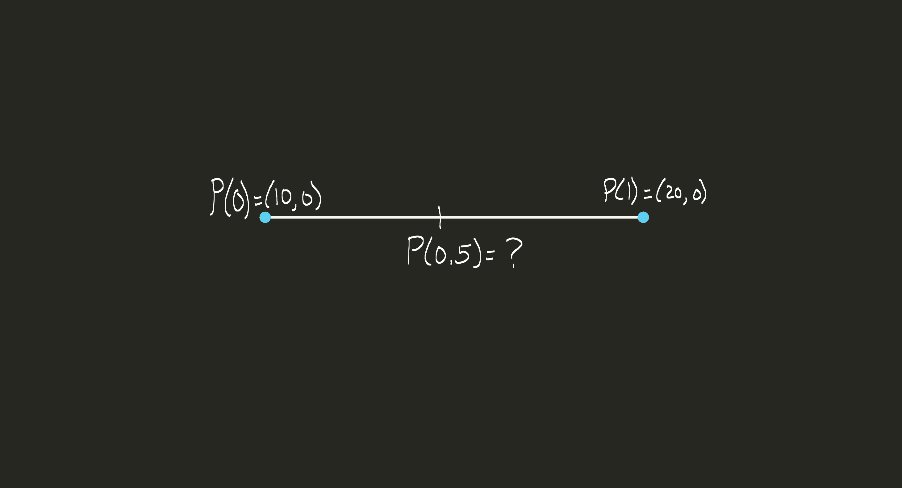
If you said 15, you guessed correctly. This makes a lot of sense to us intuitively, but what is our brain doing behind the scenes? We can abstract this into an equation pretty easily, we are simply doing:

$$(20 – 10)t + 10$$

If we abstract this one more time, we can say more generally that:

$$P(t) = (P_1 – P_0)t + P_0$$

Now we have one equation that can give us any line based off of two points. Let’s rearrange this equation to look like \(P(t) = P_1t – P_0t + P_0\). We can factor out \(P_0\) and we get an equation that looks like this:

$$P(t) = P_1t + (1 – t)P_0$$

Now that the equation looks like this, we can actually intuit what is happening behind the scenes. We are actually taking a weighted average between \(P_0\) and \(P_1\) which gives us our result. It will be helpful to think of a Bézier curve as a weighted average between all the control points.

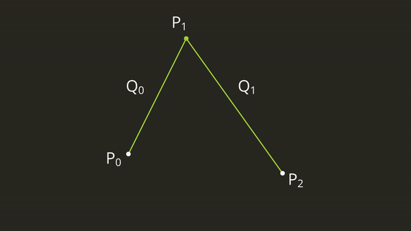
This is great, but this still doesn’t help us figure out how to find a curve where a third point is the control point. Well, imagine that we now have a third point, and we want to draw a curve that “bends” toward that control point. When we define a Bézier curve we want points \(P_0\) and \(P_2\) to have equal weight in how it bends towards \(P_1\). How can we do this? Well let’s draw two straight lines, one from \(P_0\) to \(P_1\), and one from \(P_1\) to \(P_2\). We know that we can create an equation \(P(t)\) for \(P_0\) to \(P_1\) and \(P_1\) to \(P_2\). Let’s call these lines \(Q_0\) and \(Q_1\). What if we just draw a third line, from \(Q_0\) to \(Q_1\), and we create an equation to interpolate between them. Well we can use our same equation as before \(P(t) = P_1t + P_0(1 – t)\) we can rewrite this in terms of \(Q_0\) and \(Q_1\), this would give us \(P(t) = Q_1t + Q_0(1 – t)\) and if we plug it all in we get:

$$Q_0 = P_1t + (1 - t)P_0$$ $$Q_1 = P_2t + (1 - t)P_1$$ $$P(t) = [1 – t](P_0(1 – t) + P_1t)) + t[P_1(1 – t) + P_2t]$$

This will give us a nice Bézier curve from 0 to 1 that goes through \(P_0\) and \(P_2\) and is “bent” towards \(P_1\). We can graphically visualize this as an interpolation between \(Q_0\) and \(Q_1\) like this:

Testing Pixels

Now that we can generate any equation for a Bézier curve using 3 points, we can find a way to see if a pixel located at some position \((x, y)\) intersects with this line \(P(t)\) going to the right. How do we check if the pixel will hit the curve? Well, let’s imagine that the point \((x, y)\) is actually the origin. We can achieve this mathematically, by simply translating each of our points \(P_0\), \(P_1\) and \(P_2\) by subtracting the position \((x, y)\). Now if we look at \(P(t)\) in relation to the origin, how can we tell if this point will intersect with \(P(t)\)?

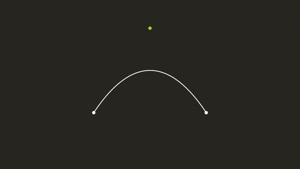
Imagine the Point as the Origin

Well, this is now just a simple question of finding the roots of this equation. We know that the equation is a quadratic function, and we should remember from Pre-Algebra that we can solve for the roots of the quadratic function using the quadratic equation. But, our formula does not look like a quadratic function, so how can we find the roots? Well, let’s rearrange our formula \(P(t)\). If we multiply all of the terms together we get:

$$P(t) = (1-t)(1-t)P_0 + (1-t)tP_1 + (1-t)P_1t + t^2P_2$$

This still doesn’t look like a quadratic function, so let’s expand the multiplication and factor out like terms next:

$$P(t) = (1 – 2t + t^2)P_0 + P_1t – P_1t^2 + P_1t – P_1t^2 + P_2t^2$$ $$P(t) = P_0 – 2P_0t + P_0t2 + 2P_1t – 2P_1t^2 + P_2t^2$$ $$P(t) = (P_0 – 2P_1 + P_2)t^2 + (2P_1 – 2P_0)t + P_0$$

Remember, a quadratic equation in standard form looks like \(y = ax^2 + bx + c\). Looking at our equation \(P(t)\), we can clearly see what \(a\), \(b\), and \(c\) are. Now, to find the roots, it’s a simple matter of setting the equation equal to 0, and plugging in the y coordinates of each point, and solving using the quadratic equation.

$$P(t) = (P_0 – 2P_1 + P_2)t^2 + (2P_1 – 2P_0)t + P_0$$ $$a = P_0 - 2P_1 + P_2$$ $$b = 2P_1 - 2P_0$$ $$c = P_0$$ $$x = \frac{-b \pm \sqrt{b^2 - 4ac}}{2a}$$

The quadratic equation will give us one, two, or no answers, depending on how many roots the function has. We can check each real root, and see if the root \(t\) is less than 0, or greater than 1. If t is less than 0 or greater than 1, it will not intersect with our Bézier curve. If one or both of the roots is between \([0, 1]\) then we will intersect with the Bézier curve. Now, we can test every pixel and see whether it will hit any of our curves simply by plugging in a few values. Using all of the combined techniques, we can now use a collection of points to define how a letter should be drawn. We can then connect these points using Bézier curves, and determine whether a pixel should be on or off by testing it and seeing how many curves it hits. Some example GLSL code might look like this:

void calculateNumberOfCollisions(
    in ivec2 p0,
    in ivec2 p1,
    in ivec2 p2,
    in ivec2 pixelCoords,
    inout float numCollisions)
{
  // Translate the bezier curve's points to the pixel's local space
  p0 -= pixelCoords;
  p1 -= pixelCoords;
  p2 -= pixelCoords;

  // Calculate the coefficients in the quadratic equation
  float a = float(p0.y) - 2.0 * float(p1.y) + float(p2.y);
  float b = float(p0.y) - float(p1.y);
  float c = float(p0.y);

  // Calculate some intermediate values for the quadratic equation
  float squareRootOperand = max(b * b - a * c, 0);
  float squareRoot = sqrt(squareRootOperand);

  // Solve for the two values of the quadratic equation
  float t0 = (b - squareRoot) / a;
  float t1 = (b + squareRoot) / a;

  // To avoid a divide by 0 error here, we clamp the value if it's close to 0
  if (abs(a) < 0.0001)
  {
    // If a is nearly 0, solve for a linear equation instead of a quadratic equation
    t0 = t1 = c / (2.0 * b);
  }

  // Add one for each valid collision
  numCollisions += t0 <= 1 && t0 >= 0 ? 1 : 0;
  numCollisions += t1 <= 1 && t1 >= 0 ? 1 : 0;
}

This function expects three points: p0, p1, p2. These points are the Bézier curve. It also takes in the pixel coordinate that we are testing. Then it translates the Bézier curve into the pixel’s local space. Next it solves the quadratic equation for t0 and t1. Finally, it adds one collision for each valid t value. If the t value is between 0 and 1, that means the pixel has collided with the Bézier curve.

Edge Cases

There are a myriad of other problems that you will encounter using this technique. Some problems to consider are what happens when a pixel hits the junction between two curves? What happens when a pixel hits a horizontal line? What happens when a pixel is on a curve? The TrueType format sets out to solve all these issues with a complicated set of instructions that are defined to handle all of these edge cases which I will not be covering.

Edge Cases

I hope that this article has showed you how something as simple as displaying text through a computer screen is not as simple as it may appear. If we take a deep dive into the mathematics behind it all though we can see how you would create a procedure to transform a series of curves into the text that you look at on a daily basis.